Prepping for Peptide Synthesis

Today, (December 13th), I went to RPI for my final research day of the first semester! Today I worked on prepping for another peptide synthesis. We are working to attach a peptide to a new linker that attaches to a resin bead. The concept is similar to another idea that I introduced in a previous post. These beads will eventually be packed into a column and used to purify biologics with the binding of the peptides on the beads.

My first job was to make 25 mL of 0.1 M NaOH from 2 M NaOH. Using the formula (M1)(V1)=(M2)(V2), I found that I would need to add 1.25 mL of 2 M NaOH and fill the rest of the volume with PBS. To carry out the dilution, I used a volumetric flask.

Next, I made 50 mL of 20% ethanol solution. To do this, I added 10 mL of ethanol to 40 mL of distilled water. After I mixed this solution, I then added 150 microliters to each of 20 wells in a well plate. After waiting for half an hour for the ethanol solution to evaporate, I added 150 more microliters to each well.

I can't believe that the first semester of my senior year is already over! I can't wait to see what's in store for me starting in January.

New Microarray Experiment

On Friday (December 6th), I finally returned to RPI! JP explained to me a new experiment that we're running. We are now running a microarray to analyze the binding of HCP proteins that we do not want to bind to the biologic that we are creating. This information will be used in the purification work I described in an earlier post.

Today, most of my time was spent waiting for the microarray slides to incubate (they had to incubate for an entire two hours!). While I waited, Doug and I adjusted the pH of the PBS he was making using a 1M NaOH solution to increase the pH to 5.5.  I then labeled the tubes for HCP and PBS solutions and the petri dishes containing the slides that would eventually be used with those solutions. Some tubes would contain 1 mL of PBS, some would contain 1 mL of HCP solution, and some would contain a mixture of half PBS and half HCP solution. After I finished labeling, I added the indicated amounts of PBS and HCP solution to the tubes.

After the tubes were all filled, Doug and I made amino acid solutions. After some practice, I'm definitely getting faster at weighing out the amino acids!

When the slides were finally done incubating, we washed them three times with the new PBS solution for 10 minutes per wash. By the time the washes were over, it was time for me to go back to Emma!

I can't wait to return to RPI next week for my last visit of the semester and see the results of this experiment!

Scanning Slides

Last Friday (November 22nd), I returned to RPI for more work! Currently, we have three methods of getting the protein that we are focusing on. The first method involves growing the protein in E-coli and lysing the cells. The other two methods involve extracting the protein from human brain cells using different buffers (which I will call buffer R and buffer T). As I have demonstrated in previous posts, our protein consists of two loops that react with each other to form a tight junction.

In all of our previous experiments, we have used only parts of the protein in microarray experiments. Today, we analyzed microarray slides that tested the entirety of the protein for the first time. We used a scanner to analyze slides that tested protein derived from each of the three methods. We scanned nine slides total. 100%, 50%, 10%, and 1% dilution for the E.Coli protein, 50% and 10% dilution for the buffer R protein, and 50% and 10% dilution for the buffer T protein. We scanned each group separately for comparison. With each group, we also scanned a control slide which consisted of no focus protein- only primary antibody- to make sure the antibody was binding specifically to the focus protein. Examples of good and bad binding of the primary antibody are seen below. The blue circles represent focus protein that was bound to the microarray, and the red represents primary antibody. We want the primary antibody to bind only to the focus protein.

For the scan, I laid each slide face down on the scanner, each oriented the same direction. I had to be careful to line them up straight right along the edge of the scanner, so later analysis using spotfinder would be easier to line up the microarray spots. 

An example slide arrangement is seen below for the E.coli slides. 

We scanned the slides first at 200 microns, then at 50 to get the most precise scan possible. After getting the images from the scanner, we imported them into a program called spotfinder to analyze the intensity of each spot. The resulting data wasn't perfect, but it was a good start! 

I will not be able to go to RPI next Friday (November 29th) due to the Thanksgiving holiday, but I look forward to returning on December 6th!

Microscopy!

Today (November 8th), we worked with cells from the blood-brain barrier using microscopy! By definition, microscopy is "investigation using a microscope." To refresh my knowledge of the microscopy processes we use, JP gave me this link to read. In our work, we used Alexa 488 and Hoechst 33342 (also known as DAPI). Before I arrived, JP fixed the cells and added the primary antibody. We had to decide whether or not to permeablize the cells before adding the DAPI. We decided to try imaging the cells without permeablization first. We added a DAPI solution to the sample, incubated the cells, and then removed the excess solution. We then washed the sample a couple times to remove excess dye.

Once the sample was ready to be imaged, we had to decide what wavelengths of lasers to use to image them. To do this, we used a program called SpectraViewer. The resulting graphs are shown below.

 The vertical line on the graphs represents the wavelength of the selected laser. The green curve represents the Hoechst 33342 and the red curve represents the Alexa 488. The shaded regions represent the region that will be recorded. We decided to use the 405 nm laser for the Hoechst 33342 and the 488 nm laser for the Alexa 488.

To image the cells, we used a Zeiss Spectral Confocal Microscope (seen in the image below). It was so cool to be able to see the cells magnified to such a high degree!

The nuclei were very clearly visible, but the staining from the Hoechst 33342 was not visible. After viewing the images, we decided that it would be necessary to permeabilize the cells and re-add the Hoechst.

I won't be able to go to RPI next week because I will be in Kansas City for my national championship horse show, but I can't wait to return on the 22nd to see the images from the cells and continue our work!

Analyzing Peptide Mapping Data

On Friday (November 1st), I did a lot of work with analyzing peptide mapping data using the Origin program. But before I get into that, JP said that the peptide formation that I prepped for last week came out perfect! Anyway, I worked with three different sets of data from the same experiment- one set of 20 peptides and two sets of 56. After copying the data from a previous Excel sheet, my first step was to change the settings of all of the odd-numbered columns to "Y-error" because it represented standard deviation data. After I had done that for all three sets of data, I adjusted the fit curves by using a one-site bind pharmacology non-linear cure fit. In that process, I had to change the k-values of every data set to 1 to standardize the fits.

 Our goal is to look at the data for each of the peptides and determine which peptides have low Kd (affinity towards the substrate) values and high R-squared values (good fit to the best-fit line). The area we are looking for is represented by the green area above. In looking at the plots, I narrowed the range to an R-squared value of 0.5 to 1 and Kd value of 3E-6 to 8E-6, and changed the data point labels to display their peptide numbers. Looking at the layout of peptides in this region, we determined that the most accurate set of data is the second set of 56, which makes sense because those peptides were made in 2012, while the peptides used in the other two sets were made in 2011.

After looking at those plots, I the plotted Peptide # vs. 1/Kd. This produced plots with many sporadic troughs and peaks. JP introduced me to the idea of curve-smoothing. Using the Kd values of the peptides, we are ideally looking for the Kd values of individual amino acids. To do this, we use averages of the Kd values of different peptides. For example, A would equal KD1, B would equal the average of KD1 and KD2, etc.

Using an Excel template that JP made for a previous experiment, I plotted averages of three up to fifteen peptides. While the fifteen-peptide averages obviously smoothed the curve the most, it is hard to determine the correct plot we should use because as the curve gets smoother, it hides certain important peaks.

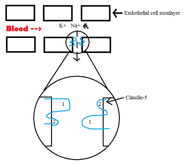
After I finished my analysis work, JP showed me some of the brain cells that he is culturing! He just started growing them on Tuesday, so they had not yet grown into a full layer of cells. They will be used to run a second trial of an experiment we did last winter, which involves testing the permeability of the blood-brain barrier by passing different sizes of sugar molecules through a layer of cells. I can't wait to continue working with the data and see where that experiment goes!

Purification Experiment Set-Up

Last Friday (October 25th), JP introduced me to another project that our lab is working on. Previously, we had two different ways to produce free peptide. First, we could grow peptides off cellulose and dissolve the cellulose in DMSO to leave the free pepide in solution. Second, we could grow peptides off of a polymer bead that has  functional groups for the peptide to attach to. These linkers could then be cut using a strong acid to produce free peptide. Now, we are working on producing peptide that grows directly off of the polymer bead, so it cannot be cleaved. Using these beads in a column, we could purify biologic. When biologic is entered into the top of the column, it would be captured by the column through the peptides. We could then elute off the biologic.

To prep for this experiment, I inserted seven specific amino acid sequences into the peptide machine program, copying each 13 times. After inserting the sequences, I used the program to see what volume of each amino acid prepped amino acids for the peptide machine. I then rounded those values up to either 5, 10, or 15 mL of solution. After determining the amount of each solution we would need, I calculated the gram amount of amino acid and mL amount of NMT to be added to make each solution. I then labeled each amino acid tube and added the specified grams of amino acid to each.

We will use the amino acid solutions that I made today to produce the seven specified peptides that I entered into the program. I look forward to returning to RPI next Friday to see what progress has been made!

HCP Assay

On Friday (October 11th), I had a variety of different tasks at RPI. My main task was to help Doug with an host cell protein (HCP) assay. In this experiment, we plan to analyze the binding of HCP to a peptide array using high-thoroughput screening of fluorescent tags. To do so, the peptide arrays will be incubated with HCP solution, primary antibody, and secondary antibody, separated by thorough washings to remove the excess solution. We will be testing different concentrations of primary antibody. The secondary antibody is fluorescently tagged, so we can screen the slides for intensity, indicating the intensity of HCP bound by each peptide.

Figure by JP Trasatti, Karande Lab, RPI

Previously, Doug printed peptides arrays onto three different slides and coated them with an HCP solution to bind the peptides. My first job was to wash the HCP solution off of the slides. This washing involves pouring off the solution from the slide and adding 10 mL of PBS to the petri dish, then rotating them for 10 minutes to wash off any excess HCP that was not bound by the peptide array. We then made the different concentrations of primary antibody and applied them to the respective slides, making sure all of the solution stayed on the slide and was evenly distributed. After an hour of incubation, we then washed the primary antibody and applied the light-sensitive secondary antibody.

While we were waiting for the primary antibody incubation, we were going to make western transfer buffer, but we did not have enough methanol. Instead, we made 2L of PBS, which is a process I have done before!

I am excited to return to RPI and see the results of this experiment, but I will unfortunately not be able to go this Friday (October 18th) due to Parents' Day.

Host Cell Proteins

On Friday (October 4th), I finally returned to RPI after missing a week! I worked with Doug (one of the undergraduates in my lab) on a project he is working on involving host cell proteins. A couple weeks ago, these host cell proteins were involved in the SDS-PAGE gel we were working on!

Previously, we have only had intensity data to analyze the amount of host cell protein (HCP) that is bound by different peptides. This is relative data, so it does not give us information about the actual amount of HCP that binds. Ideally, we want to find a peptide that has a high affinity for the target protein we are looking to purify, but low intensity of HCP (the green square in the graph below). We do not want the result to be in the red square, indicating high affinity for the target protein, but high intensity of HCP.

Doug is working to quantify the amount of HCP that is bound by the peptides. To do so, he is printing different concentrations of HCP on nitrocellulose (negatively charged paper) 3X5 microarrays. These spots of known HCP amount will then be analyzed for intensity to determine a standard curve. The standard curve will then be used to determine the unknown (amount of HCP) for the peptide data.

My first job was to pipette 80 microliters of 6 different concentrations of HCP into their specified positions in the printer well-plate. We then cut the nitrocellulose paper into slide-shaped pieces and taped them onto the printer so they wouldn't move during printing. When we were setting the heights for the printer needle, one of the pieces of nitrocellulose cracked, so we had to untape and redo the nitrocellulose. Once we finally had the printer set up, we set the first round of printing to run, and we found that the middle spot on the second slide was not printing. We then reconfigured the needle heights and made each height tighter to the nitrocellulose. As we continued to run the machine, we realized that the needle was popping up every time it went to print on the first slide, so we had to tap the needle down every time it was positioned on the first slide. Because the printing was taking so long, we decided to only do 10 runs instead of the original 20 runs planned. Even the 10 runs took over 2 hours to complete!

I look forward to returning to RPI next week to see what data they collected from this experiment!

More Amino Acids

Last Friday (September 20th), I returned to RPI for more lab work. I had a shorter day today because I had to leave early to go to Massachusetts for a horse show. This week, I continued to work on preparing amino acid solutions. I finished the rest of the 20 amino acids that I started to make last week! These amino acid solutions will eventually be used in microarray experiments.

I will not be able to go to RPI next Friday because I am participating in a program at Cornell, but I'll look forward to returning on October 4th!!

Data Preparation and Amino Acids

Yesterday (September 13th), I went over to RPI for more work in the lab. I got to see the gel I prepared last week! Unfortunately, the gel turned out useless because it had too many metal ions which caused there to be what was basically an extended row of dye instead of separated bars. The gel was still helpful, though, because now we will not attempt any more gels with those types of solutions!

My first job for the day was to compile some of the data from our previous Claudin-5 microarrays. For each of our past experiments, we have pixel intensity data for the resulting microarrays. At this point, we want to compile all of the past data to be able to look at it as a whole. On JP's computer, each past experiment has it's own folder, so I copied an .mev converter file into each folder. After doing so, I opened the .mev converter file and all of the .mev files for a certain experiment, and I moved all of the data into the converter file. After doing so for every experiment, the .mev converters were ready to run, and they will be run by next week!

My second job was to prepare tubes to make amino acid solutions. I labeled each tube:
Three-letter code (one-letter code)
Mg amino acid to be added
mL solution to be added

After doing this for all 20 amino acids, I then began to add the specified amount of each amino acid to its specified tube.

I can't wait to continue my research next Friday!!

Preparation for an SDS-PAGE Gel

Last Friday (September 6th), I went over to RPI for the first time during this school year! My primary job for the day was preparing for an SDS-PAGE gel. For this gel, we are working with a specific protein of interest.Ultimately, the gel will analyze the bands of the null solution (which does not contain the protein of interest, but contains other host cell proteins (HCPs)) versus the bands of the solution that contains the protein of interest (in addition to the other HCPs). To do this, we are working with different types of protein solutions. First, there are the null solution and the protein of interest solution which are both prepared at 1X and 10X concentration. The different concentrations will ultimately lead to different width bands. Also, there are 10X desalt solutions for both the null and protein of interest. In the original solution, the buffer contains metal ions that can affect how the bands are displayed in the gel, making them appear blurred. In the desalt solutions, the buffer has been exchanged to PBS to eliminate the metal ions and get cleaner bands. Once the gel is run, we expect to see something like the simplified gel below. We expect to get certain bands from the null solution that represent the bands of the HCPs, and we expect to get those same bands from the protein of interest with the addition of an extra band that represents the protein of interest (represented in red in the image).

Today, to prepare for running this gel, I first made the Tris/Glycine/SDS buffer by combining the stock solution with water, mixing the buffer, then putting it on ice to keep it cold (keeping the buffer cold allows for sharper bands in the gel). Next, I made the blue Laemmli sample buffer by combining the stock solution with β-mercaptoethanol (BME). I then labled the solution tubes with the different solutions and added 20 micro-liters of Laemmli buffer to each sample. After each sample was allocated into its respective tube, I denatured the protein solutions in a heat bath for one hour. To prevent the sample tubes from popping open in the heat bath, I wrapped each sample with parafilm (which ultimately caused them to stick together). After the proteins were denatured, I spun the samples, and set them aside to cool. I then set up the gel equipment.

The gel was then ready for JP to run later in the day! I can't wait to see the results when I return to RPI on Friday!

Back to Senior Year!

Although I did not blog this summer, I continued to work in the lab at RPI! Over the summer, I learned so many skills that I can't wait to apply to my work this school year. After my experience at RPI last year, I could not be more excited to start another year in the same lab. Spending an extended period of time in the lab has allowed me to continue to practice different skills with the machinery and materials in the lab, so I am now capable of doing much more than when I first started last Fall!  This year, I hope to keep perfecting my skills and to learn new ones. I hope to continue to get a solid feel of what it's really like to work in a college lab before I head off to college myself next year!

Looking Back

Last October, I said that I was looking forward to my internship because I wanted to learn new things and experience a professional environment. After an amazing year, my internship has allowed me to do so much more than that. From the very beginning, I was integrated right into JP's lab and given as many hands-on jobs as possible. My only challenge was believing that I was capable of doing all JP thought I could! This year, I have had so much fun working with new equipment and processes in an environment that was not only professional, but encouraging for me to get involved. I have taken part in many different microarray experiments as well as smaller side projects, and I have had the opportunity to both set up experiments and analyze the data. Presenting my work to the school at the end of the year was an amazing opportunity for me to share my experiences with the Emma community. (Just to prove how supportive my mentors are, both JP and Dr. Karande came to Emma to see my presentation!) I would not trade my internship experience for anything, and I strongly encourage any Emma girl to do an internship if she is dedicated to the sciences and ready to experience what could come after Emma. My only suggestion for the program is to meet with the other interns more often so we can routinely share our experiences. My advice to future interns is don't be afraid to get involved. Everything may be overwhelming at first, but trust your mentors and you will have an amazing year! While it may sound like I am saying goodbye to my internship, I actually have the incredible opportunity to continue working in JP's lab over the summer. I thank everyone involved for an incredible year, and I can't wait to see what's next. Thank you for reading my blog! 

Presentation

Last Wednesday (May 1st), I presented the research from my internship to my school in our Student Achievement Assembly. I am so proud to be an example for all of the amazing work the Emma interns do, and presenting my work gave me a unique opportunity to expose the secret lives of the STEM girls. It was a great way to end a great year!

New Permeability Experiment!

This Tuesday (April 23rd), I went to RPI for another day to set up a new experiment! This experiment is similar in process to the experiment I was introduced to on December 11th. However, in that experiment, we were testing the natural permeability of the blood brain barrier, and this time we're testing the permeability of the blood brain barrier with our manufactured loop-2 protein added! As in the other experiment, the set up is two wells (one inside the other) with a filter on the bottom of the inner one separating the two, as seen in the figure below. On this filter, there is a monolayer of brain cells to represent the blood brain barrier.

We will have many of these setups in order to test solutions with different size molecules. We will be testing solutions with molecules that are 4 kDa, 10 kDa, 20 kDa, 40 kDa, and 70 kDa. All of these molecules are dextrans, or different size sugar molecules. For the normal type blood brain barrier that we tested earlier, the permeability to size curve looked like the black line below.With the peptide modulator that we have made, we hope to make the curve look like the red line below.

Today, we made the peptide solution to be added to the cell monolayer. We had to make sure that the protein was at a certain concentration in the PBS solution, so we used a Nanodrop spectrophotometer like the one below. The Nanodrop spectrophotometer analyzes the concentration of the solution by measuring absorption. 

We also changed the media of the cells to a non-phenol-red media. The cells are usually cultured using phenol-red media because it is a pH indicator. When the media is exhausted and needs to be changed, the media changes from purple to yellow. However, using this media in our experiment could alter the results. To change the media, we used a vacuum line to remove the old media and then added the new media to both the top and bottom wells. Once all of the materials were ready, we added the peptide solution and dextran solutions to the wells and started the experiment. 

I can't wait to see the results!

Graph Irregularities

This Tuesday (April 14th), I went to RPI to analyze data from another microarray affinity experiment. Affinity is the attraction to a substance, in this case a labeled protein. We used two different blocking buffers in this experiment. On one microarray, we used the BSA (bovine serum albumin) that we usually use with the microarrays. On the other microarray, we used a crude mixture (protein broth) from the company whose protein we are trying to purify, which contains contaminants as well as the protein of interest. Both of these microarrays were tested in concentrations from 1 nM to 3.5 nM. We graphed the data as intensity vs. concentration, where high intensity meant high affinity toward the printed peptide. The expected intensity vs. concentration graph would look like the graph below.

However, I looked through all of the graphs and found irregularities like the ones shown below. The third irregularity is especially strange because the intensity is very high at low concentrations, but very low at high concentrations.

After I finished recording the irregularities in the graphs, I looked at the kD values for the same experiment. I looked at each peptide sequence in relation to its position on the protein, and recorded the high and low kD values for each region.

Also, there was a vendor fair in our building today! We took a break to go look at the new technology, including movers, shakers, and much more. Overall, it was a lot of fun!

New Project

This Tuesday (April 9th), I finally went back to RPI to continue my research! JP introduced me to a new project that the lab is starting. Due to property concerns, I can't go into it in detail, but it has to do with a protein that binds to transferrin, which then attaches to a receptor on endothelial cells. This protein can then be moved through the cell into the brain via receptor mediated endocytosis. To produce this protein, we are going to use a cloning vector in E. Coli, which we will remove the protein from via osmotic shock. Each of the target proteins have a flag sequence attached. This flag will allow us to use an antibody that binds to the flag to purify the protein.

Our first project, explained earlier, is involved with opening a pathway between endothelial cells to allow transport into the brain. This new project also focuses on transport into the brain, but it is involved with making a pathway through endothelial cells.

Microarray Model

Last Tuesday (April 2nd), my mentor was out of town, so I did not go to RPI. However, my mentor gave me a project to work on for the week! We are working on taking concepts involved in our research and turning them into hands-on craft projects for children in grade school through high school. My project is to come up with a craft demonstration of how a microarray works. A microarray is a glass slide that usually contains nucleotide or amino acid probes that bind certain molecules. My concept is to use Velcro to demonstrate the binding of the printed peptide propes to molecules in the solution the microarray is exposed to. In our research, we use amino acid probes to make a microarray that consists of  56 peptides, each in a 3 by 3 matrix. For my demonstration, I am planning to use cardboard to represent the glass slide of the microarray. For the peptide probes, I am planning to use adhesive circles of Velcro. Some of the Velcro circles will be the hook side, and some will be the loop side. For the binding molecules, I will use Styrofoam spheres that have one kind of Velcro, hook Velcro for example, attached. These "molecules" will then bind to some of the "peptide probes," but not to others. To simulate the coating of the microarray, the "slide" will be put in a box, or "petri dish," and the "molecules" will be poured in. The box will then be moved in circular motions like it is on a rotator. After being "coated," the excess balls will be pored out of the box, and only the bound "molecules" remain attached to the microarray.

We also discussed having a second part to the activity using a "mixture" with varying sizes of molecules to demonstrate epitope mapping. Overall, we hope to use this demonstration to aid learning about microarrays, protein interfaces, purification of solutions, and peptide engineering.

Missed Weeks :(

Last week (March 5), I was unable to go to RPI because I was sick. This week (March 12), my mentor was on spring break, so I could not go this week, either! For the next two weeks (March 19 and March 26), I will be on spring break, so I will not be going to RPI. I can't wait until I can go back and continue my research!

More PBS and Data!

This Tuesday (February 26th), I ventured to RPI to continue my work in the lab. This week, I was again tasked with making PBS solution. As I explained in a previous entry, PBS (phosphate buffered saline solution) can be used to dialyze protein solutions. PBS is made by combining 15.52 mL of 1M K₂HPO₄, 4.48 mL of 1M KH₂PO₄, 2 L of distilled water, and 11.6 g of NaCl. After mixing these contents, I had to raise the pH to 7.4 using 1M NaOH base. After creating a pH of 7.4, I filtered the PBS using a bottle-top filter with a vacuum attached, like the one shown below.

After finishing the PBS, my next job was to work with the data from the concentration experiment I helped set up last week. First, the organization of slides on the Origin program was different than the actual setup, so I had to convert the data to accurately represent its respective slide. Once I reorganized the data, I was able to run the program to create graphs and calculate the 1/kD and R2 values for each piece of data. Luckily, the experiment worked almost perfectly! Each of the graphs looked like the one shown below, which was the graph we predicted last week before the experiment was run. 

I looked at every graph and recorded the numbers of the graphs that did not seem to fit the data points as well as the others. I then copied the origin data twice into an excel sheet and sorted the data according to 1/kD value and R2 value. Most of the R2 were 0.9 or above, which means that the data followed the curve very well. I tried to find a correlation between the graphs with worse 1/kD values and worse R2 values, but there did not seem to be an obvious correlation between the two. I color coated the data in both sorting sets according to different R2 value ranges. There were no R2 values in the blue range! 

• Set 1- green- 0.95+
• Set 2- yellow- 0.9-0.95
• Set 3- red- 0.7-0.9
• Set 4- blue- less than 0.7

This coding allowed me to look for further correlation between 1/kD value and R2 value, but there still appeared to be no correlation between the two. 

I can't wait to work with the data more next week!

AAAS Convention

Last weekend, a couple of the other interns and I had the opportunity to go to the AAAS (American Association for the Advancement of Science) Convention in Boston!

We were able to choose what lectures we wanted to go to, and we spent all day listening to different scientists talk about their work! I attended lectures including:

• Language as an Adaptation to the Cognitive Niche - Steven Pinker
• More Than Pretty Pictures: How the Process of Making Science Images and Graphics Clarifies Understanding - Felice Frankel 
• The Robotic Moment: What Do We Forget When We Talk to Machines? - Sherry Turkle 
• Resurrected Ancestral Proteins: Fundamentals and Applications - Joseph Thornton 
• Stroke Research: New Concepts and Innovative Solutions - Moll Shoichet, Constantino Iadecola, and Stephen Meairs 
• The Connectome: - William Seeley, Jeff Lichtman, Mark Bear, and Steve Petersen 

I really enjoyed the lecture about resurrecting ancestral proteins because it used some of the same technology that I am learning to use in my internship! I also really enjoyed Felice Frankel's lecture because it combined science and art in a really interesting way! We were also able to visit different booths that were set up, including one that focused on enantiomers. An enantiomers are a pair of molecules that are mirror images of each other. They have identical chemical properties, but they can react very different in biology! For example, +Limonene smells like oranges and -Limonene smells like pine! We were able to build these molecules (below). 

Overall, it was a great experience to be immersed in the world of science! It definitely inspired me to pursue my next steps in becoming a scientist! 

Concentration Experiment!

Today (February 19th), I went over to RPI to continue my work in the lab. Since last week, slides of peptide arrays were printed using the amino acid solutions I made. Today, I helped use these printed slides to set up and run an experiment. In this experiment, the goal is to determine what part of loop 1 of the Claudin-5 protein in the endothelial cell tight junctions reacts with loop 2 on the opposite side of the junction. These loops can be seen in the diagram below. 

In this experiment, we are using a solution of 90% unlabeled peptide and 10% TAMRA labeled peptide. The TAMRA binds to terminal alkynes via a copper-catalyzed click reaction, and it is fluorescent red. The fluorescent tagging is useful in determining where the peptide binds to the printed 56 peptide array via intensity analysis. In this experiment, There are 10 slides containing 56 printed peptides each. Each of the slides will be exposed to different concentrations of TAMRA tagged peptide, the highest being 500 mM and the lowest being 100 mM. On the highest concentration slide, we expect to see all of the dots tagged at a high intensity, and on the lowest concentration slide, we expect the TAMRA tagged peptides to bind only to the highest binding proteins on the slide. To analyze the intensity of each peptide binding spot, it will be scanned into a computer program, and the intensity will be evaluated using pixels. This data will then be plotted on an intensity vs. concentration graph. We expect the data to resemble the graph shown below, with the intensity increasing as the concentration increases and eventually plateauing. This graph will then be used to find 1/2 of the plateau intensity, and identify the concentration of that intensity. This value will be used to find the Kd, or the affinity of the peptide towards the substrate. 

In my work today, I helped to set up this experiment. Overnight, the slides were placed in individual petri dishes and coated with BSA (Bovine Serum Albumin) to prevent the peptide from binding with the blank space on the slide where no peptide dots are printed. My first job was to wash the excess BSA off of the slide with PBS. The PBS solution I used today was actually the PBS solution I made on one of my first visits to the lab! To wash a slide, I first poured the excess BSA out of the petri dish. Then I added 10 mL of PBS to the petri dish, making sure to not add it directly onto the slide to avoid forcefully removing BSA from the slide. I then repeated this process for the other nine slides, and then put on them on a rotator for 10 minutes. This process was repeated three different times to ensure that all of the excess BSA was removed. 

While the slides were on the rotator, JP and I did calculations to determine the volume of unlabeled peptide, TAMRA peptide, and PBS solution to put on each slide. The amounts were different for each slide because the concentration of TAMRA peptide was different. To add the peptide solution, we used the properties of surface tension, as in adding water droplets on a penny. However, the slide had to remain wet, so it made the process more difficult. First, I poured the PBS solution off of the slide. Then, JP dried the sides and bottom of the slide to allow us to use the properties of surface tension. While JP was drying the slide, I dried the petri dish with Kimwipes. The slide was then put back in its labeled petri dish. We then added the specified concentration peptide solution to the slide, making sure it was evenly dispersed and that none went over the edge of the slide. We then repeated this for each of the slides, using the different concentration peptide solutions. After all of the slides were coated with their specified solutions, we covered them with black paper because the TAMRA is light sensitive. The slides are going to sit and be slowly rotated for three hours. 

I can't wait to see the results from this experiment next week! It should give us useful information going forward in our research. It was very interesting today to see different activities I have done in the lab come together. The amino acid solutions I made last week were used in the printing of the peptide slides, and the PBS solution I used today was the solution I made! I look forward to continuing my research and learning more new procedures!

Amino Acid Solutions

This Tuesday (February 12th), I went to RPI for my weekly internship meeting. This week, I was in charge of making amino acid solutions to be used in the peptide printer. First, I had to calculate the volume of the solution that needed to be added to each amino acid powder. I was given each of the 20 amino acids in their powder form in separate tubes. The mg of powder in the tube was labeled on the side, along with the three letter abbreviation of the amino acid. I was also given a sheet of the dilution concentrations (mg and mL) for each amino acid. Using these numbers, I had to calculate the unknown, which was the volume of solution that needed to be added to the amino acid powder. For example, if the given concentration was 2 mg / 10 mL, and the tube contained 0.5 mg of powder, I would need to add 2.5 mL of solution. The concentrations for each amino acid were different, so I had to do that calculation 20 different times. After my calculations were finished, I went to the lab next door to use the fume hood to create the solutions. To do this, I used an Eppendorf that measured in microliters. The maximum volume that the Eppendorf could hold was 1000 microliters, or 1 milliliter, and the average volume I needed to add to the tubes was 4 mL, so I had to add the solution in smaller amounts. After each amino acid, I had to change the tip of the pipette to prevent contamination between amino acids. After adding the specified volume of solution to each of the 20 amino acids, I took the amino acid solutions back to our lab. There, I used a vortexer like the one shown below to dissolve the amino acid powder in the solution. Some were much easier to dissolve due to their polarity. These solutions will be used in the peptide printer to print arrays of peptides for future experiments. 

I'm looking forward to finding out what I will do next week!

Modeling Peptides

This Tuesday (February 5th), I went to RPI to continue my project from last week. Last week, I identified possible α helix binding sites on the protein. SInce last week, JP has worked on using the color coded model to come up with amino acid sequences that would form an α helix structure and bind to one of the sites. My job was to test the possible structure of the amino acid sequences by entering them into a program called PEP-FOLD. This program uses the amino acid sequence to identify possible  reactions between the amino acids that would make the protein's secondary structure. Ideally, the amino acid sequence we are looking for should have an almost perfect α helix secondary structure in order to bind well with the binding site on the protein. The figure below was the most successful α helix model we made. 

We also built the amino acid sequence using the MOE software. We set the program to make the sequence into the ideal α helix shape to determine where the bases would be located on the α helix. This allowed us to align our α helix sequence with its binding site on the protein model to identify the possible reaction sites and see how we could change the amino acid sequence to improve the binding. 

Overall, my work today really increased my knowledge about amino acid sequences and protein structure. I look forward to continuing to work on this project!

Protein Structure

Yesterday (January 29th), I went to RPI for more interesting analysis! We started with a summary of protein structure, which was really cool because we recently learned about protein synthesis and structure in AP Bio, so it was really cool to apply it to research! Protein structure is divided into different levels of structure. Primary structure (1˚) consists of the amino acid sequence of the protein. To form secondary structure (2˚), different amino acids that are not adjacent in the sequence can react and cause twists in the amino acid strand. The two common secondary structure forms are the α helix and the β pleated sheet. Today, as I will explain later, I focused on α helices. Tertiary structure (3˚) is formed when the secondary structure folds on itself, forming a three-dimensional structure. Finally, the quaternary structure (4˚) gives the protein form and function by adding molecules such as sugars and phosphates or combining different proteins together. Below is a diagram showing the different protein structures.

Source: Madison Technical College Lab Manual on Protein Structure

Today, my task was to look at a protein structure using MOE software. We are looking for a site to bind another molecule, especially the α helix sites. Two α helix forms can aggregate like a zipper, like the bindings of two spiral notebooks. I identified all of the different helix sites and recorded them by amino acid sequence numbers. After they were identified, I color coded them on the model so we could see where they were located in the three-dimensional surface structure of the protein. It was so interesting to see the relationship between the amino acid sequence and the final structure of the protein! It added a lot to my knowledge of protein structure and allowed me to apply something I learned in class.

As usual, I can’t wait to see what comes next!

Analyzing Data!

Today (January 22nd), I went to RPI for another day of interesting work! Today, I analyzed the data from the experiment I was introduced to on December 11th. To summarize the experiment, we were analyzing the size of particles that can normally pass throught the blood brain barrier, using a set up with two wells, one inside of the other (seen below). Twenty wells were tested. Ten had the dextrans added to the apical (inner) chamber, two each for the five different dextran solutions (4 kDa, 10 kDa, 20 kDa, 40 kDa, and 70 kDa). The other ten had the dextrans added to the basolateral (lower) chamber, two each for the five different dextran solutions. Further explanation of this experiment is given in my blog post from December 11th.



The data from this experiment came from solution samples taken at various times over a 25 hour time period. These samples were then scanned and analyzed according to their fluorescent signal. The dextran molecules contained Fluorescein Isothiocyanate (FITC), so the more fluorescnet signal the sample had, the greater the concentration of dextrans in that sample.

To analyze the data, I copied the data from the scan program into a program called Origin. There were three separate scans, so I had to average the data from the three. I then plotted the data for Concentration vs. kDa. After detecting errors in the beginning and end of the graphs, I trimmed the graphs to get a more accurate linear fit. After trimming the graphs, I calculated the r-squared values for each kDa. 4 kDa had by far the best fit. 10 kDa had the worst, and then the r-squared values increase for the 20, 40, and 70 kDa. After examining the Concentration vs. kDa data, I plotted the data for Concentration vs. Time for each of the 20 wells. For every well, the concentration increased over time. This is because as the time increases, more of the cell monolayer dies off, and more dextran molecules are allowed through the barrier. From the starting concetration values, it was evident that the larger molecules started with a lower permeability.

Overall, I had a very interesting day of analyzing data! I can't wait to see what's coming next week. 

Passaging and Protein Structure

Today (January 15th), I went to RPI for my first day of lab work of the new semester! Today was full of really interesting new things. First, JP showed me how to culture tissue, particularly the practice of passaging. Passaging is the process of moving some cells from a previous culture to a new growth medium to allow them to continue to grow. The first thing we had to do was spray everything down with ethanol. Everything must be sterile when working with the tissue, so all materials were sprayed, including our gloves. Next, we got the tissue culture out of the incubator, which maintains the CO₂ level and temperature similar to that of the human body. Before passaging the tissue, I was able to observe the culture under the microscope. The proteins that had been previously cultured were connected in a chicken pattern, and they were attached to the surface of the container with linkages that kept them in place. First, the media was removed from the container with a vacuum line. Then, 10 mL of PBS solution was added to the container to remove dead cells and remove the Fetal Bovine Serum (FBS) that inhibits the enzyme Trypsin from acting on the cells. Trypsin functions to cut the anchor linkages that connect the protein to the container, causing them to float around, which is not wanted while the tissue is being cultured. The PBS was then removed from the container with the vacuum line. Next, 1 mL of Trypsin was added to detach the cells from the container. After the Trypsin was active in the container for a few minutes, I observed the cells in the container again, and they were now floating islands of groups of cells. Next, FBS was added back into the container to re-inhibit the Trypsin. This mixture was then transferred to a conical vile to be spun down in the centrifuge. Once the centrifuge was balanced, it was spun at 1000 rpm for 5 minutes to make a protein pellet separate from the media. While the vile was being spun, we prepared a new container, and labeled it as passage #25 of the cells. 35 mL of new media were then added to the new container. After the vile was done in the centrifuge, the old media was drained from the vile using the vacuum line. We then added 1 mL of media to the vile to re-suspend the protein pellet by using the pipette up and down until the protein pellet broke up and dispersed in the media. 100 microLiters of the suspension were then added to the new container, and it was agitated to spread the cells around the surface of the container. The passage was then complete, and we re-cleaned everything with ethanol and put the new culture in the incubator.

After passaging, JP introduced me to a new computer program for modeling proteins. The program displayed both the amino acid sequence and the three-dimensional structure of the protein. My job was to search through the entire amino acid sequence to highlight certain amino acids that are important to the function of the enzyme. Once I highlighted the amino acids in the sequence, I also highlighted the corresponding structures on the enzyme that those amino acids code for. The purpose of this activity was to show the position of the binding site of the protein structure. After locating the binding site and seeing its structure, we looked at how the signal molecule (which is a sugar) binds to the binding site. This program was really interesting because I am learning about protein synthesis and structure in AP Biology right now!!!!

I can't wait to return next week and find out what's next!

Cleaning Up

12.18.12

On Tuesday December 18th, I went over to RPI for the last time before winter break. Because RPI was wrapping up their work as well, there were not any new experiments to be set up or new data to interpret. My day was full of cleaning and organizing the lab equipment and bench spaces. Also, I was able to see our lab's liquid nitrogen container, which was really cool! I can't wait to return after break and continue with our work.